on QED
a photon has zero electro-magnetic charge, but can display properties of either positive (right hand spin, wavelength) or negative (left hand spin, particle) polarity. For the purposes of this brief exposition I will refer to photons as having both positive and negative charge simultaneously, such that they cancel each other out.
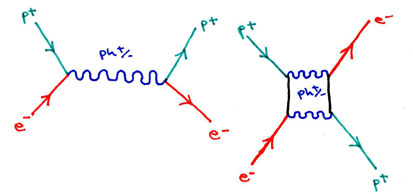
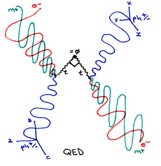
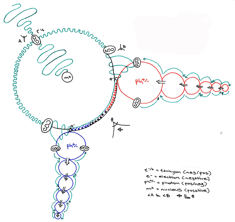
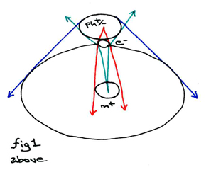
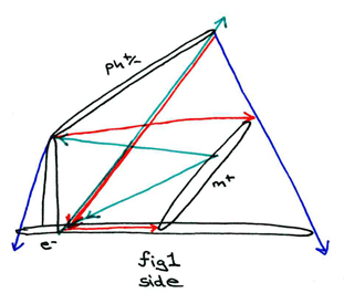
Here we see the standard and modified Feynman diagrams for the annihilation of a positron (p+) and an electron (e-) to form a photon (ph+/-). In the original Feynman, the temporary annihilation period results in altered spin vectors for the electron and positron from before to after their duration in combination as a photon. The modified version shows how a pair of photons can be created by the same annihilation of a single positron and electron pair; I have modified this to show that the spin vectors of each can possibly remain unaltered from before to after their duration in combination as the particle-wave photon. We should observe that, in both Feynman models, the electron accounts for the negative characteristics (left hand spin, wavelength) of the photon, while the positron accounts for the positive characteristics (right hand spin, particle) of the photon.
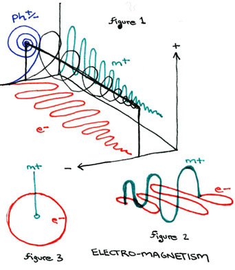
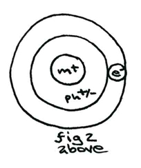
In the diagram labeled "ELECTROMAGNETISM" we see three figures. The third figure is the standard model of the electron's negative charge (e-) orbit around the positive charge magnetic dipole (m+). In figure two, we see this diagram modeled over a time duration, and seen at an angle, so that we can see that the electrical charge's orbit is perpendicular to the precession of the magnetic dipole (the electrical and magnetic forces operate at right angles to one another). In figure 1, I have borrowed a model depicting the orbit of earth around the sun over time to demonstrate why the electical and magnetic wavelengths operate at right angles to one another, and why photons operate at a third right angle to both forces. The model indicates that the unification of these three-dimensional forces lies in the spiral wavelength of a fourth-dimensional force.
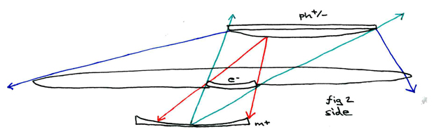
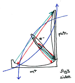
Now, to return to the Feynman diagram structure, in this diagram I depict the zero-duration event of a photon striking an electron. This diagram displays how the EM field's spin vectors can possibly remain unaltered from before to after the collision, and that the photon's spin vectors can possibly be altered from before to after the collision. The duration of their annihilation is marked by the exchange between the spin vectors of two tachyons operating at right angles to one another. The point of annihilation of the photon and electron is a temporal (charged) singularity, while the point of intersection of the two tachyons is a gravitational (non-charged) singularity. According to this model, whenever a photon and electron strike one another, a tachyon travelling from and a tachyon travelling to the gravitational singularity at the center of our local universe exchange directions.
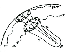
Here is a model showing how this can be accomplished even for a photon in one galaxy and an electron in another when each passes into the event horizon of a black hole. An electron travelling in the same direction parallel to a photon can actually cross paths and annihilate with that photon through the wormhole of the event horizon such that the photon's and the electron's spin vectors can actually switch places over astronomic distances.
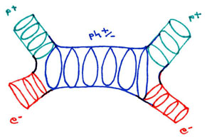
The modified model of the Feynman diagram for particle-antipartical annihilation has become the standard model for string-theory. Here we see that vibrational harmonic resonances surround the quantum field of particle-wave duality of the electron, positron and photon. These vibrational harmonic resonances (called superstrings) are comprised of extra dimensions which have not "expanded," and which surround and conserve the three-spatial dimensions of our local universe.
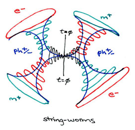
In my model of string theory we see how the electrical (e-) and magnetic (m+) charges of the EM field combine to form a photon before and after the annihilation of a photon into two tachyons operating at right angles to one another. Once again, the point t=empty-set represents the gravitational singularity, while the entire diagram itself represents a temporal singularity. Because energy is entering and exiting the model simultaneously, we see that a temporal singularity (such as occurs upon the collision of a photon and electron) is the same thing as a wormhole.
Discuss this section on the forums
further musings on QED
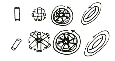
In this image we see two possible ways to rotate an electromagnetic dipole.
In the top figure we rotate the dipole centrifugally around an axis intersecting the midpoint of the dipole and operating at right angles to it. This process is sped up until the positive polarity and negative charge reverse so rapidly that the result is a dually charged electromagnetic torus.
In the lower figure we rotate the dipole centripetally around one end of the dipole. The resulting torus will be either positive or negative around the outside, and the opposite charge in the center, essentially a monopole.
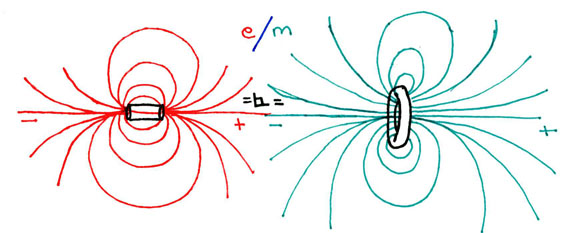
In this image we see the electrical field lines of a dipole and the magnetic field lines of a torus. It should be noted that, should the dipole and the monopole convector be swapped, the phase portrait of the field lines for each will be the same, even though now the dipole will be magnetic and the monopole electrical.
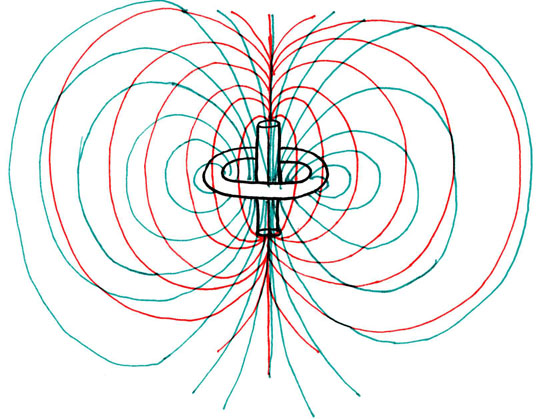
When the dipole is inserted through the monopole it becomes clearer how the field lines of the electromagnetic force act at right angles to one another. Along the poles of the dipole the forces are oriented parallel such that they overlap perfectly. However, around the middle of the dipole, as well as surrounding the circular monopole of the torus, the field lines operate at right angles to one another.
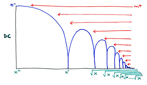
Direct Current:
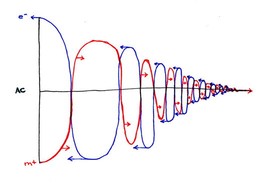
Alternating Current:
possible QED experiment
musings on the photo-electric effect
advanced QED
a magnification:
Discuss this section on the forums
Modeling elipses using cones and photo-optics
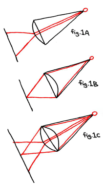
In figure 1 we see the focus of light shown from the point of a cone through different types of lenses at the base. The convex lens in fig.1A refracts the light from a single concentrated beam into a more diffuse field. The concave lens in fig.1B refracts the light from a diffuse beam into a single concentrated point. In fig.1C we see the combination of these effects rendered by a dual-sided convex lens.
In figure 2 we see the same cones from a different angle so as to better view the way the light is refracted through their lenses. Here, the vertical diaganol line perpendicular to the conical bases is shown from a 45° angle above the cones and between the bases and the perpendicular plane. For simplicity's sake, the bases of the cones are depicted as circular, and consequently, the planes reflecting light from them as being a planar elipse, however any shape area can be substituted for the conical bases, and consequently any angles and vertecis of the lens. The elliptical nature of the reflecting surface will be better deomnstrated from the angle depicted in the next diagram. The types of lens A, B, C remain the same as in diagram 1.
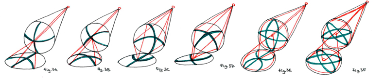
In figure 3 we see the same cones from 45°s above and 45°s to the right. Whereas in figures 1 and 2 we saw only one version of each of the three cones, in figure 3 we see two versions of each of the three cones. The different versions depict two perpendicular arcs drawn on the surface of the lens and seen from two different positions in the rotation of the conical bases. For example, fig.3A and fig.3B depict perpendicular arcs on the convex lens seen at 90° and at 45° of rotation, or rather, at perfect vertical/horizontal orientation (3A) and at diaganol orientation (3B). The rest of this figure should be clear.
Discuss this section on the forums
modeling photo-electric QED with lenses
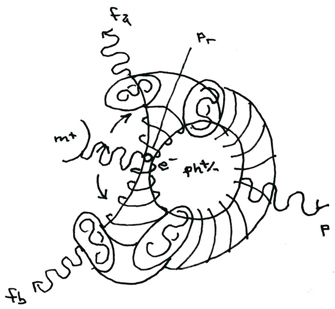
Here we see the standard model of photon-electron collision. The photon (ph+/-) is depicted at the temporal singularity of it striking the electron (e-). As the two make contact, the event horizon of the orbital shell probability cloud of the electron collapses down into the charged particle of the electron. This can be depicted by using angles of incidence to portray the angular momentum of the electron's orbital vector.
The red lines here indicate the angle of incidence of the electron in the "shock" wave probability well created by the impact of the photon. Notice that thered lines, otherwise parallel, are warped into intersection in the presence of the photon. The green lines represent the angle of incidence for the photon relative to the nucleus (m+) at the center of the atom. Notice that it collapses sharply such that the electron's probability cloud is shown to conserve the photic momentum vector. The blue lines depict the relative paths for the photon's projected trajectory following the temporal singularity of its striking the electron. The photon's projected trajectory will combine with or deduct from the prior angular momentum of the electron, and here we see this dual probability expressed as being similar to the double-slit experiment.
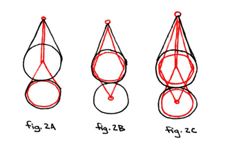
Here we see the photon, electron, and nucleus depicted as conic sections. The photon is an ellipse, the nucleus is a circle, the electron's orbital shell is the base of the cone, and the electron itself is a parabola extending between the conic base and the blunt elliptical top. These are all depicted in black lines, while the relative incidence vectors from above are presented according to the same red, green and blue angles. Here, the parallelism of the photic and electric "shock" wave point wells is indicated, and the photon, electron and nucleus depicted at their relative angles to one another. The right angle, for example, between the parabolic electron point and the magnetic orbital conic base represents the orthogonality of the electromagnetic force.
This picture is essentially looking at the first figure from a yet different angle. It has all the same components, (ph+/-), (e-) and (m+) and their incidence vectors. However, here the idea expressed in looking at the first figure from the side of seeing the constituent components as flat (rather than, as tradionally, spherical) is enhanced one step further by their portrayal as a set of lenses. (Ph+/-) is a convex lens, (m+) is a concave lens, and (e-) is a convex/concave lens. Here we see the initial incidence vectors transformed into refracted beams of light.
What is significant about this model is that, by depicting the spherical components as relatively flat lenses, and their relationships as refracted beams of light, we are creating an experimentally verifiable model by which to look at tachyons as gravitic. For example, the red lines of the electron incidence vector here become a beam of light (gravitic tachyons) projected from the photon lens, through the electron lens, and onto the nucleus lens. From there, the same beam of light is reflected back (the green lines) through the electron to the photon. Finally, the same beam of "light" is bounced back down to cast the relative "shadow" of the electron's orbit from the lens of the photon. Note that all of these "beams" remain consistent to the angles of incidence in the first diagram, but that now, rather than spherical or conic section constiutent components, we are modeling the same notions with lenses.
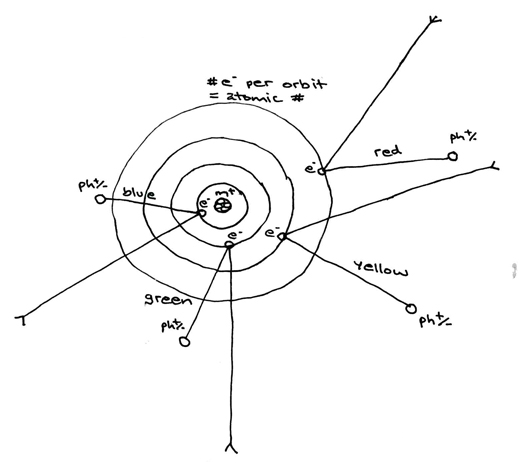
So, returning from this again briefly to the spherical (Bohr) atomic model, we see the photon above connecting with the electron (right) in its orbit (outer circle) around the nucleus at the centre. Compare this with the side view model using lenses and note how the incidence vectors can be interpolated logically.
Here is a somewhat more complex model using all the same constituent components as we just saw in figure 2. Here the convex photon, concave nucleus and orbital trajectory are all represented as intersecting at a right angle. Although this situation is nt the one that occurs naturally when a photon strikes an electron (the photon itself never coming into direct contact with the nucleus), this diagram is nonetheless helpful in assisting us to see the peculiar warping of the photo-electric incidence vector (the blue lines) under different hypothetical conditions. In other words, if the angle of orientation between the photon and the nucleus were to prove to be orthogonal (based on, for example, the forces for which each is a particle carrier being oriented perpenidcularly to one another, as is the case with the electromagnetic force), then the temporal singularity of the photon-electron collision could be expressed as the sum over the difference of the two opposite probabilistic projected trajectories, one taken by the photon, the other by the electron (again, the lines in blue).
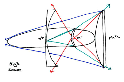
This diagram represents the same orientation of the constituent components as the last, and holds all the same referential labels and relative relationships as the preceding. This diagram is possibly, however, the clearest in its ability to illustrate the incident vectors as refracted "beams" of gravitic tachyons.
Discuss this section on the forums
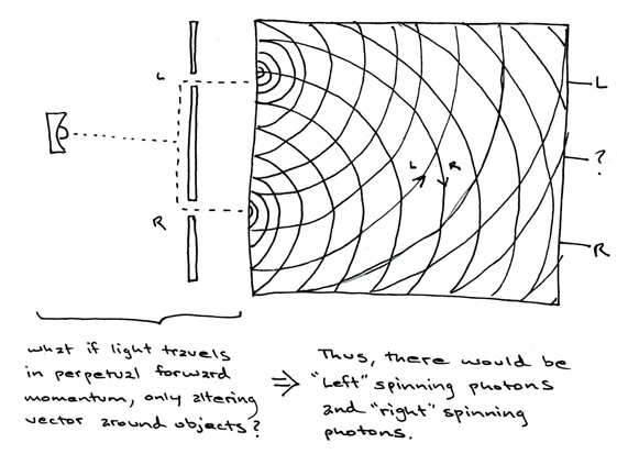
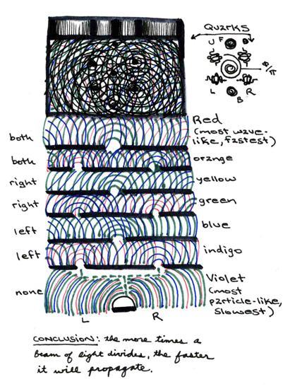
the double-slit experiment