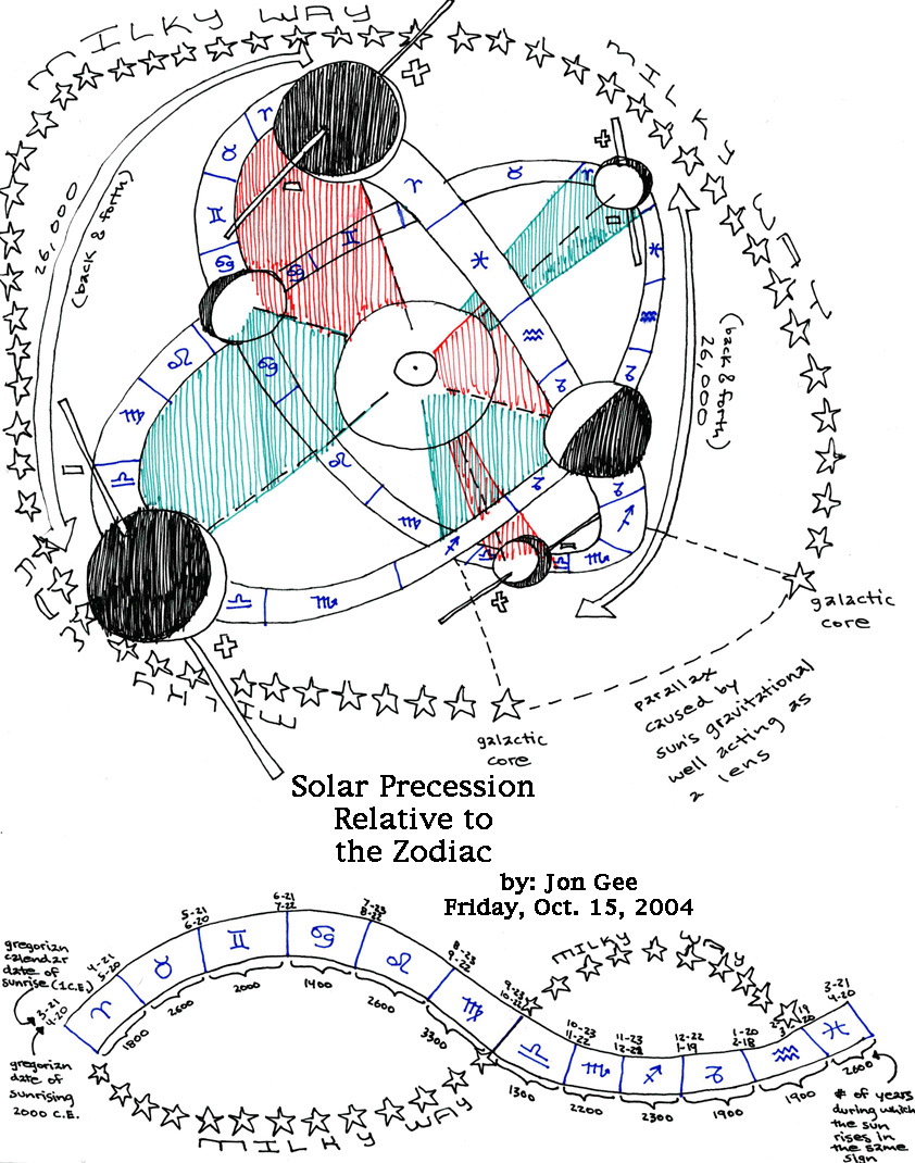
This picture I have chosen to link to instead of image. The reason for this is that it is a somewhat large picture. It is really two diagrams on one page.
In the top diagram we see the earth (shadowed by night) rotating around the sun, clearly marked, at the center. The orbital path of the earth around the sun is depicted as the zodiac, although the ecliptic plane of the zodiac, technically, does differ somewhat from our own current equator. The poles of the earth are shown on the outer four stations, and labeled positive and negative. It should be noted that the positive and negative stations reverse depending on whether the earth is ascendant or descendant to the equator of the sun. Because the planet's orbit is reckoned to be more elliptical than oblate, the red and green shaded ratios on the diagram represent the porportions of Kepler's Third Law of motion by which to guage the duration of time taken, and thereby the speed, of the planet in one of said positions. The time it takes for the orbital plane of earth around the sun to precess from the plus to the minus electromagnetic polarity is approximately 26,000 years, or about twice the time it takes for the geographic pole to precess around in one full rotation. The reason for this will be explained in the following images.
At the bottom of the page is another diagram, however what it depicts is clearly labeled.
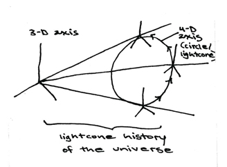
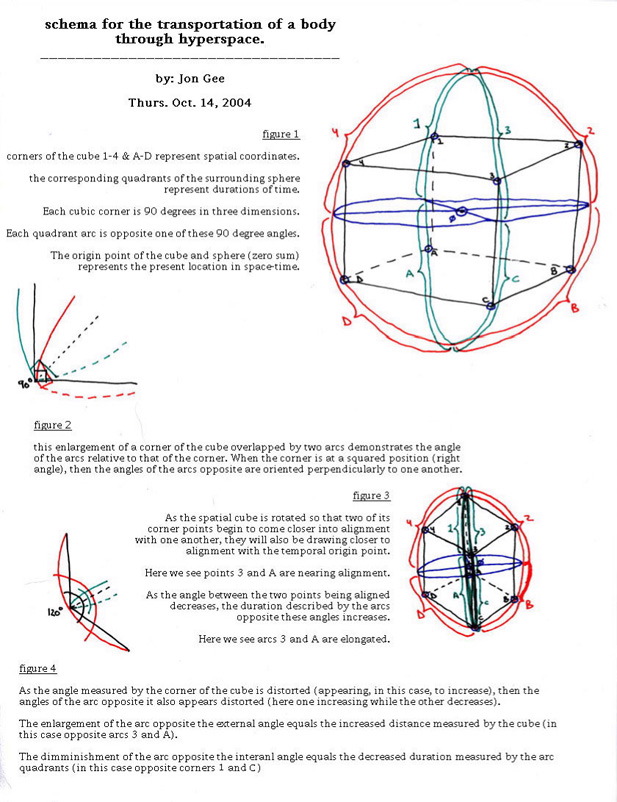
to measure the relativity of three points at one time, construct one three-dimensional axis for all three, then trace out the point of intersection for one random angle from each point, and construct an axis system for this point. To measure a duration, follow the same procedure for a single point at three different times.
The circle of the base of this cone will always be a measure of the fourth dimension. It acts as an angle at which the three other directions meet, a plane connecting them all as a tetrahedron. For example, in a 3-sphere, this angle is confined to 45 degrees of the circumeference of the sphere for 3 right angles.
----------------------------------------------------------------------------------------------------------------We can depict and thereby easily understand the three standard accepted dimensions comprising the spatial component of our continuum. We model this as the intersection at right angles of three planes, and depict it using diagrams such as the 3-star described above.
However representing the fourth dimension, whether we understand it spatially or temporally, or spatially and temporally, is not quite as easy.
For example, it is possible to understand four spatial shapes by depicting the possible shadows that they cast into the third dimension, and then modeling these, usually as flat diagrams drawn in the second spatial dimension. However, these 3-space shadows of 4-space objects, no matter how thoroughly we can model them in either stasis or motion, are limited as 2-spatial diagrams, as well as being limited to representing the 4-space shapes only at certain angles. For example, a cube seen from above a corner casts a hexagonal shadow on a sheet of paper, and so, too, is the 3-space tesseract the shadow of only one possible position of the, otherwise much more difficult to visualise, 4-cube.
Another way of modeling the fourth dimension is by examining 3-spatial shapes over time. Let us understand the temporal dimension as beiing the measure, perpendicular to the three intersecting planes of 3-space, of a 3-spatial object from itself. For example, imagine a cube sitting on my desk. The difference between this cube and itself can be rendered as the passage of time. Of course, in this model, we cannot see any immediate difference between one state of the cube and another from one moment to the next. So, if we want to model dynamic change over duration we must work with moving parts. Consider, instead of the cube, a gyroscope sitting on my desk. Now, as the gyroscope is set in motion and spins, there is an immediately visualisable difference between itself in one state and itself in another from one moment to the next. Hence, we can use motion as a measurement of the temporal direction, which, again, operates at a fourth right angle to the standard intersection of planes in 3-space.
Now, ideally, to consider the full scope of the fourth dimension, we should combine the shadow effect of one dimension being visualisably diagramable on the next dimension beneath it, AND the measurement of motion as being perpendicular to the 3-spatial matter upon which it acts. So, for example, let us consider the following two diagrams.
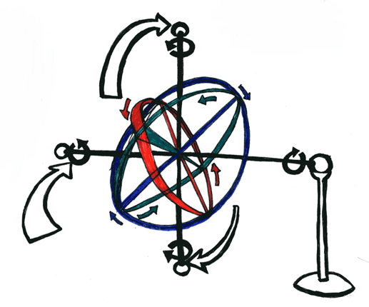
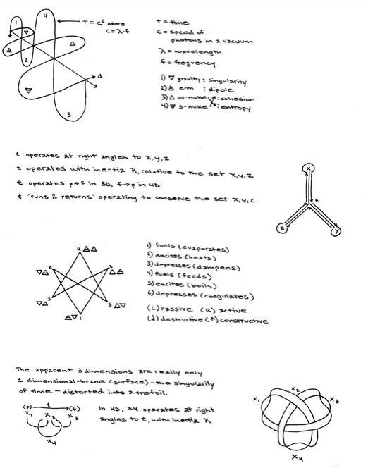
The first measures several different directions of motion on the model of the gyroscope. Here we see that the three planes intersecting at right angles may be depicted as the axes of three great arcs. Each great arc has its own orientation of motion, and the momentum caused by the motions of the combined three great arcs causes further dynamic rotation to occur. In the case of this diagram, that motion is depicted by the insertion of a 2-space axis at 45° between the perpendicularly oriented axes of the three great arcs. As the great arcs revolve around the origin point of these conjoined axes, their motion creates the momentum that drives the rotation of the 2-space axis. The 3-arcs revolve and the 2-axis rotates. To add even one more step of motion to the model, I have pinioned the entire gyroscopic contraption upon a stable pivot, such that the 3-arcs revolve, causing the 2-axis to rotate, causing the whole gyroscope to revolve around the pivot point. (for reference, the revolution of the great arcs is depicted by the three colour arrows, the rotation of the 2-axis by the solid black semi-circular arrows, and the revolution of the contraption around the pivot by the black outlined white arrows.) This diagram maps the confluence of nine directions of motion, and if the pivot point had been rendered such that, rather than being stable, it followed a precessional concourse (imagine the pivot-beam tracing out a circle around the base of its stable stand), then the diagram would model motion in at least ten different directions. Of course, it is equally easy to continue adding motion in as many different directions as possible, however for the purpose of this exposition we needn't worry about the implications of doing so.
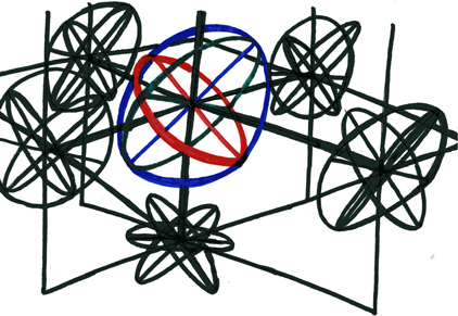
The second diagram depicts the same essential model, that being the gyroscope, as well as the shadows that it casts in five of the six cardinal directions. It should become evident upon consideration of this diagram that only three of these shadows are actually necessary for a thorough examination of light's effects on the model, the other three shadows merely being equal and opposite mirror images of the first three. For the sake of brevity the motions of these shadows are not depicted, however it is hoped that the viewer of this diagram should be able to piece these together for themselves.
Discuss this section on the forums
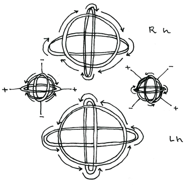
There are four basic stations of motion for the tripartite gyrsoscope. These represent different spin states for the 3 great arcs of the gyroscope. The right hand (Rh) and left hand (Lh) spin states are simple spinors with only one direction for all three great arcs. These create simple vortecis in a fluid medium, where the rotation of the spin of the gyroscope drives the liquid substance into a simple vortex in the center of the gyroscope. The other stabe positions of the gyroscope involve either one or two of the great arcs moving in an opposite direction from the other(s). These, depicted on the left and right of the diagram, orient themselves with positive and negative positions where the fluid medium disrupted by the motion of the gyroscope will be drawn toward the positive positions and away from the negative positions. In the model on the left, the positive poles are positioned relative to the static horizontal great arc, while in the model on the right, the positive poles are positioned relative to the static position of the greater vertical arc. Because there are dual polar positions for the other models, we can call them scalar rather than spinor vector motions.
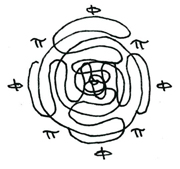
Here we see the product sum over histories for the fluid dynamic medium perturbated by the motion of the three-arced gyroscope. This model fits the motions of the scalar polar model on the left (above), where the greater vertical arc remains static and the other great arcs move in opposite directions relative to one another. I have taken the liberty of labeling these spirals by the short-hand notations for PI (the arithmetic spiral) and PHI (the exponential spiral).
----------------------------------------------------------------------------------------------------------------this information is all © 2004 - Jonathan Barlow Gee
LINKS: